QuakeCast: Benchmarking Classical and Machine-Learned Models of Aftershock Sequence Evolution
Every number in this document is generated from persisted experiment
artifacts (artifacts/) and checked against them by scripts/claims.py;
tables are regenerated by scripts/paper_tables.py.
Abstract
We benchmark classical and machine-learned forecasts of aftershock counts on 14 real sequences from USGS ComCat, INGV and GeoNet (36,622 aftershocks above a pre-registered completeness magnitude), issuing every forecast forward in time and scoring it by its full predictive distribution. Pooled over sequences, each held out in turn, the Epidemic-Type Aftershock Sequence model is the strongest forecaster: +0.171 nats per event over the Omori–Utsu law ([+0.096, +0.307]), above it on 14 of 14 sequences. Gradient boosting trained across other sequences also beats Omori (+0.130), but its gain lives almost entirely in the first three days (+0.243), when the still-incomplete catalog leaves a young sequence's own decay law unidentified — Omori fits sit on their search bounds in 15 of 42 of those windows. After a week no learned model beats Omori with an honest negative-binomial spread, and learning within a single sequence never helps (−0.056). For locations, a cell-level boosted model does not reliably beat an adaptive kernel density estimate (+0.045, [−0.019, +0.106]). This is a characterisation study of sequences already under way; it makes no claim about predicting mainshocks.
1. Question and scope
After a large earthquake, the rate of aftershocks decays roughly as a power of time and their locations cluster around the rupture. Statistical models of this behaviour — the Omori–Utsu law for the rate, the Gutenberg–Richter law for magnitudes, and the Epidemic-Type Aftershock Sequence (ETAS) model that lets every aftershock trigger its own — are the basis of operational aftershock forecasting. This study asks one question:
Can modern machine learning improve the characterisation of how an aftershock sequence evolves, relative to established statistical baselines?
"Characterisation" is meant literally. QuakeCast forecasts the number and the spatial distribution of aftershocks above a completeness magnitude after a mainshock has already happened, over horizons of one to thirty days. It does not predict the time, place or size of any future mainshock, it is not an operational forecasting system, and nothing in it should be read as one.
Five sub-questions structure the work: (Q1) does ML improve aftershock-rate forecasts, (Q2) does it improve spatial density forecasts, (Q3) how does it compare with the classical laws and models, (Q4) how stable are the results across sequences, and (Q5) does generalisation fail across tectonic regimes?
2. Data
2.1 Catalogs
All events come from authoritative public catalogs through the FDSN event web-service standard; no event, magnitude, location or time is synthesised.
| Region | Provider | Service |
|---|---|---|
| California and northern Baja California | USGS ComCat (networks ci, nc) | earthquake.usgs.gov/fdsnws/event/1 |
| Central Italy | INGV | webservices.ingv.it/fdsnws/event/1 |
| New Zealand | GeoNet / GNS Science | service.geonet.org.nz/fdsnws/event/1 |
For every event the pipeline keeps the provider event identifier, origin time, latitude, longitude, depth, magnitude, magnitude type, contributing network, review status where the provider reports one, and the catalog of origin. Raw responses are cached compressed and hashed by query so every run is reproducible offline.
Conventions validated in code. ComCat GeoJSON times are epoch
milliseconds in UTC and coordinates are ordered [longitude, latitude, depth]; FDSN text times carry no zone designator and are UTC by
specification. Validation rejects any event outside the valid latitude and
longitude ranges (the signature of a coordinate swap), rejects
timezone-naive times, drops events without a magnitude or location, and
removes duplicate identifiers. Depths may be negative (above the datum) and
are kept as reported. Magnitude types are heterogeneous — SCSN reports
mostly coda (mc) and local (ml) magnitudes for small events — and are
retained rather than silently homogenised; §7 discusses the consequence.
Why regional catalogs outside the US. An initial survey drew fifteen
candidate sequences from ComCat alone. Outside the United States ComCat
holds only the largest events: the 2016 Kumamoto sequence has 73 events
inside its aftershock zone, the 2016 Norcia sequence 54. Such catalogs
cannot support any rate model, and a cross-regime comparison built on them
would measure catalog quality rather than tectonics. Italian and New
Zealand sequences are therefore taken from INGV and GeoNet. No public FDSN
access to the Japanese (JMA), Taiwanese or Chilean national catalogs was
used, so those regions are out of scope; the excluded sequences and the
reason for each are recorded in sequences.EXCLUDED.
2.2 Sequences
Fourteen mainshocks were resolved against their providers' live services;
verify_registry re-checks every identifier, origin time, location and
magnitude against the catalog before a run. Magnitudes are each agency's
preferred value, so the same earthquake can differ between agencies
(Darfield 2010: ComCat Mw 7.0, GeoNet Mw 7.2).
| Sequence | Catalog | Mw | Mc | Events ≥ Mc | Window (days) | Truncation |
|---|---|---|---|---|---|---|
| Landers 1992 | ComCat | 7.3 | 2.5 | 3,679 | 0.5–365 | — |
| Hector Mine 1999 | ComCat | 7.1 | 2.6 | 1,069 | 0.5–365 | — |
| Ridgecrest 2019 | ComCat | 7.1 | 2.0 | 4,729 | 0.5–365 | — |
| Northridge 1994 | ComCat | 6.7 | 2.4 | 1,051 | 0.5–365 | — |
| El Mayor–Cucapah 2010 | ComCat | 7.2 | 3.0 | 1,076 | 0.5–365 | — |
| Loma Prieta 1989 | ComCat | 6.9 | 1.3 | 4,140 | 0.5–365 | — |
| San Simeon 2003 | ComCat | 6.5 | 2.1 | 2,150 | 0.5–281 | Parkfield 2004 zone overlaps |
| South Napa 2014 | ComCat | 6.0 | 1.2 | 607 | 0.5–365 | — |
| Parkfield 2004 | ComCat | 6.0 | 1.2 | 2,666 | 0.5–365 | — |
| L’Aquila 2009 | INGV | 6.1 | 2.1 | 2,183 | 0.5–365 | — |
| Amatrice 2016 | INGV | 6.0 | 1.8 | 3,912 | 0.5–64 | in-zone M5.9 (Visso) |
| Norcia 2016 | INGV | 6.5 | 2.3 | 3,778 | 0.5–365 | — |
| Darfield 2010 | GeoNet | 7.2 | 2.8 | 4,641 | 0.5–365 | — |
| Kaikōura 2016 | GeoNet | 7.8 | 3.2 | 941 | 0.5–365 | — |
Table 1. The benchmark sequences. Mc from the protocol of §3; events are
above Mc, inside the zone and inside the window. Generated from the
artifacts by scripts/paper_tables.py.
2.3 Sequence definition
Sequence membership is a modelling choice, so each part of it is explicit and varied in §6:
- Zone. A circle about the mainshock epicentre whose radius is the Gardner & Knopoff (1974) distance window for the mainshock magnitude (77 km for Landers, Mw 7.3). The Wells & Coppersmith (1994) subsurface rupture length is the alternative rule.
- Window. From
t0 = 0.5days to 365 days after the mainshock. - Truncation rule (pre-registered). The window closes just before the earliest of (a) a later in-zone event with M ≥ M_main − 0.5, which starts a new sequence rather than continuing this one, and (b) the origin of another registered mainshock whose zone intersects this one, so that no two benchmark sequences share target events.
- Trigger history. Events up to 30 days before the mainshock (foreshocks) are kept as ETAS triggers but never as targets. Ridgecrest 2019, whose Mw 6.4 foreshock came 34 hours before the Mw 7.1, is why.
- Local geometry. Spatial models work in kilometres on an azimuthal-equidistant projection centred on the epicentre, which preserves distance from the centre exactly (tested against the haversine distance to machine precision). Kernels in degrees would be silently anisotropic on the ground.
3. Catalog completeness
Aftershock models are only meaningful above the magnitude at which the catalog records essentially every event (Mc). Immediately after a large mainshock, small events are hidden in the coda of larger ones, so Mc is elevated for hours to days — short-term aftershock incompleteness (Kagan 2004; Helmstetter et al. 2006; Page et al. 2016). In the Landers catalog, maximum-curvature Mc falls from 2.7 in the first days to 1.8 after about fifty days, and the b-value estimated at M ≥ 2.8 in the interval 0.2–0.5 days is 0.70 — an incompleteness artefact, against 1.02 at M ≥ 3.2.
Completeness estimators disagree. On synthetic catalogs with a gradual detection ramp (tests/test_completeness.py), maximum curvature (Wiemer & Wyss 2000) and the 90 % goodness-of-fit level underestimate the true threshold, while 95 % goodness-of-fit and b-value stability (Cao & Gao 2002) land near it. A single goodness-of-fit pass can also succeed by chance on a sparse upper tail: the Parkfield catalog, complete near M 1.0–1.2, yields a spurious 2.3 in one time bin.
Mc protocol (version 3, fixed before any model comparison). (1) Split (t0, t_end] into eight log-spaced time bins, merging any bin with fewer than 100 events into the next. (2) In each bin, the per-sample estimate is the goodness-of-fit Mc at R ≥ 95 %, else at R ≥ 90 %, else b-value stability; the bin's Mc is the median of that estimate over 200 bootstrap resamples (Woessner & Wiemer 2005 recommend bootstrapping Mc). (3) The sequence Mc is the largest bin Mc, rounded up to 0.1, so the catalog is complete at that level throughout the window — including its early, worst-recorded part. Mc is a property of the catalog, fixed once per sequence and shared by every model; because estimators still disagree by about 0.5 early in a sequence, raising Mc is a primary robustness axis (§6) rather than something tuned.
b-values use the Aki (1965) maximum-likelihood estimator with the Shi & Bolt (1982) uncertainty.
4. Models
Every model forecasts the number of above-Mc aftershocks in a window (T, T + h] from events with time ≤ T only.
4.1 Classical baselines
-
Poisson (mean rate) — a constant rate over (t0, T]. Deliberately naive; reported so that improvement over "no decay at all" can be told apart from improvement over the physical models.
-
Persistence — the rate over (T/2, T] carried forward. A stronger naive reference.
-
Omori–Utsu — λ(t) = K/(t + c)^p fitted by maximum likelihood on (t0, T], with K profiled out analytically and a multi-start search over (c, p). Recovers known parameters from simulated catalogs to within 1 % in p (tests/test_omori.py).
-
ETAS — temporal ETAS (Ogata 1988): λ(t) = μ + Σ_{t_i<t} K e^{α(m_i − Mc)} (t − t_i + c)^{−p}. Maximum likelihood with an analytic gradient (checked against finite differences to 10⁻¹⁰). Forecasts come from Monte Carlo simulation of the branching process (500 catalogs), with magnitudes drawn from the fitted Gutenberg–Richter law truncated at the mainshock magnitude, because future aftershocks trigger further aftershocks and no closed form exists. With the true parameters the forecaster is calibrated on simulated catalogs (probability-integral-transform χ² p = 0.88; 90 % interval coverage 0.90). Parameter recovery on simulated catalogs of about 900 events is within 1–9 % for all five parameters.
Two ETAS variants are reported. ETAS (primary) fixes μ to the pre-mainshock background rate — the median yearly count above Mc in the zone over the ten years before the mainshock, which uses past data only — and constrains the branching ratio over 365 days to at most 0.99, the condition under which the process is non-explosive. ETAS (free) estimates all five parameters without constraint. Both decisions were made from diagnostics, before any model comparison: early in a sequence the free fit can trade an enormous background rate against a runaway p (at T = 3 days for Landers it returned μ = 68 events/day with p at its upper bound), and a supercritical fit produces forecasts that grow without bound.
4.2 Machine-learned models
All learned models use the same 21 history features computed from events
with time ≤ T (ml/features.py, which raises if it is handed a later
event): counts and rates in log-spaced trailing windows, an empirical local
decay slope, a fit-free 1/t extrapolation, mainshock and largest-aftershock
magnitude relative to Mc, time since the largest aftershock, the b-value so
far, recent mean magnitude, and spatial spread. Targets are counts;
losses are Poisson.
- Poisson GLM — L2-regularised Poisson regression.
- Gradient boosting (GBM) — LightGBM with a Poisson objective.
- GBM-hybrid — the same booster trained with the Omori forecast as an offset, so it learns a multiplicative correction to the physical model rather than the whole rate.
- Poisson MLP — two tanh layers (32 and 16 units), Adam, weight decay, early stopping; the neural representative. Recurrent, convolutional, transformer and neural point-process models carry far more parameters than a pool of a few thousand forecast windows from fourteen sequences can identify, so they were not fitted.
Two training regimes answer different questions:
- Within-sequence. At origin T the model trains only on examples from the same sequence whose target window closed by T — (o′, o′ + h] with o′ + h ≤ T on a fixed grid of 60 log-spaced sub-origins. Early in a sequence there are too few such examples (fewer than 24), and the model abstains.
- Cross-sequence. The model trains on other sequences and forecasts an unseen one. Three training pools: pooled (every other sequence), chronological (only sequences whose mainshock came first — no calendar-future information), and other region (only sequences from a different region group). Pooled + within adds the target's own closed windows (transfer with local adaptation).
5. Evaluation design
Forward-in-time only. Forecasts are issued at 15 log-spaced origins (1–240 days) for horizons of 1, 7 and 30 days, every model refitted at every origin on data up to that origin. No split is random. Leakage guards are enforced in code and tested (tests/test_leakage.py): feature builders reject future events, training windows must close before the origin, and the features at an origin are provably invariant to anything after it.
Scores. Each model is scored against the full predictive distribution it implies. Deterministic-rate models (Poisson, persistence, Omori, the learned models) imply a Poisson count; ETAS forecasts are over-dispersed and are scored with a negative binomial matched to the simulated mean and variance. Scoring ETAS with a Poisson would penalise it for honestly reporting the spread of a cascading process; scoring Omori with a negative binomial it never claimed would flatter it. Reported: the log predictive score (strictly proper; Gneiting & Raftery 2007) and the per-event information gain over Omori; MAE and RMSE on log₁₀(count + 1); 90 % interval coverage; the randomised probability integral transform for calibration (Czado, Gneiting & Held 2009); and the CSEP number test (Schorlemmer et al. 2007; Zechar et al. 2010) per window. Comparisons use only windows where every compared model issued a forecast. Uncertainty on information gain within a sequence comes from a moving-block bootstrap over windows (forecast windows are autocorrelated); across sequences, from a cluster bootstrap over sequences, the unit across which generalisation is asked.
Spatial. Every spatial model outputs a density over the same 2 km grid covering the zone, normalised to one, with an identical 0.1 % uniform floor mixed into every model so one unexpected epicentre cannot score −∞. Models: uniform; Gaussian kernel density with a forward-cross-validated bandwidth; nearest-neighbour adaptive kernel density; an ETAS-style kernel (Omori-time-weighted power-law kernels about past events, temporal parameters from that origin's ETAS fit, kernel shape by forward cross-validation); and a cell-level LightGBM. All tuning uses pseudo- forecasts that closed before the origin. The score is the mean log density at the observed epicentres.
6. Robustness design
Each variant changes one choice: Mc raised by 0.3 or 0.6 above the protocol; t0 of 1 or 2 days; radius scaled by 0.5, 1.5 or 2; the Wells–Coppersmith radius rule; a 180-day window; truncation off; foreshock lookback off. Variants run at lighter settings (eight origins, 200 ETAS simulations) and are compared with the primary design at the same light settings, so settings never confound a design effect.
6a. Changes made after the first Landers run (disclosed)
The design in §§3–6 was fixed before the multi-sequence runs, but the first full Landers run was used as a validation pass, and it changed five things. Each change was justified by a defect found in that run, not by a better score, and is listed here so a reader can discount accordingly.
- Spatial tuning horizon. Forward cross-validation needs a pseudo- forecast whose window closed before the origin; for 30-day windows none exists until day 30.5, so every early spatial model silently fell back to fixed defaults. Tuning now uses the longest shorter horizon (7, 3 or 1 day) with closed windows.
- ETAS-kernel shape grid. With γ ≤ 1 the largest mainshock kernel was ≈ 8 km wide, far below the scale of a M7 rupture; γ = 1.5 was added.
- ETAS optimiser. The subcritical fit moved from SLSQP to a reparametrisation in which the branching ratio is a box constraint (K solved from n = 0.99·sigmoid(z)) with an analytic gradient. On Landers this reached the same log-likelihood at every origin (to 0.01), which established that the degenerate early fits (α and p on their bounds) are genuine maxima of a flat likelihood, not optimiser failures.
- Dispersion twins. A "+ NB spread" twin was added for every Poisson-predictive model (§5), after Landers showed Omori's Poisson intervals covering 42 % of outcomes at the 90 % level while ETAS won on log score despite worse point accuracy. The twin separates skill in the mean from honesty of the spread.
- Snapshot maps. A variable-shadowing bug meant no spatial density maps were saved in the batch run (scores were unaffected). The maps were recomputed with the same procedure and are marked as recomputed; a regression test now covers it.
7. Results
7.1 Catalogs and completeness
Protocol completeness differs by two magnitude units across the fourteen sequences (Table 1): the dense Northern California network records Parkfield and South Napa completely near M1.2, while Kaikōura's catalog is complete only above M3.2. At a b-value near one, each magnitude unit is a factor of ten in event counts, so absolute counts and absolute scores are not comparable across sequences. Every comparison below is therefore made within a sequence — every model on the same windows — and only then pooled.
7.2 One sequence, completely: Landers 1992
Landers (Mw 7.3) was benchmarked first, and in full, before any other sequence was run. Above Mc 2.5 the catalog holds 3,679 aftershocks in the window, and the classical models were scored on 45 forecast windows (15 origins × 3 horizons).
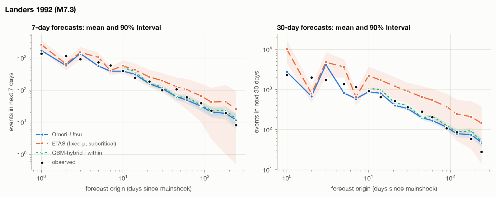
Figure 1. Landers 1992: 7- and 30-day forecasts (mean and 90 % interval) against the observed counts.
Point accuracy and probability disagree. The Omori–Utsu law has the most accurate mean: its error in log₁₀(count + 1) is 0.125, with almost no bias (−0.033). But its Poisson intervals are far too narrow for clustered counts — the 90 % interval covers 42 % of outcomes and the number test rejects 53 % of its forecasts. ETAS has a worse mean (error 0.263, bias +0.190: it over-forecasts) yet a better log score, an information gain over Omori of +0.135 nats per event ([+0.012, +0.237]), because its simulated predictive distribution is honest about spread: coverage 67 %, number-test rejections 27 %.
Spread explains part of it, not all. Giving Omori a negative-binomial spread fitted to its own closed forecasts raises its coverage to 71 % and gains +0.016 ([+0.001, +0.050]) — real but small next to ETAS. ETAS's advantage is concentrated in the first days: on the 30 later windows where the learned models also forecast, ETAS gains only +0.006 and Omori with the NB spread +0.012.
Within-sequence learning does not beat the law. Trained only on windows of the same sequence that had already closed, the Poisson GLM scores −0.020 ([−0.044, +0.010]) against Omori, the Omori-offset GBM −0.019 ([−0.040, +0.006]), and an unconstrained GBM −0.051 ([−0.084, −0.004]), the one interval that excludes zero.
Early fits are not identified. The Omori fit finished on its search bound at 4 of 15 origins and the primary ETAS fit at 3 of 15, all in the first week, when the still-incomplete catalog makes the rate look flat. The forecasts from those fits remain usable; the fitted decay parameters do not.
Cascades run away at long horizons. Issued once at day 30 for the rest of the window, Omori forecasts 793 events against 1,176 observed; the subcritical ETAS forecasts 9,381 (90 % range 4,010–16,576). A branching ratio held just below one still compounds over eleven months.
7.3 Fourteen sequences, each held out in turn
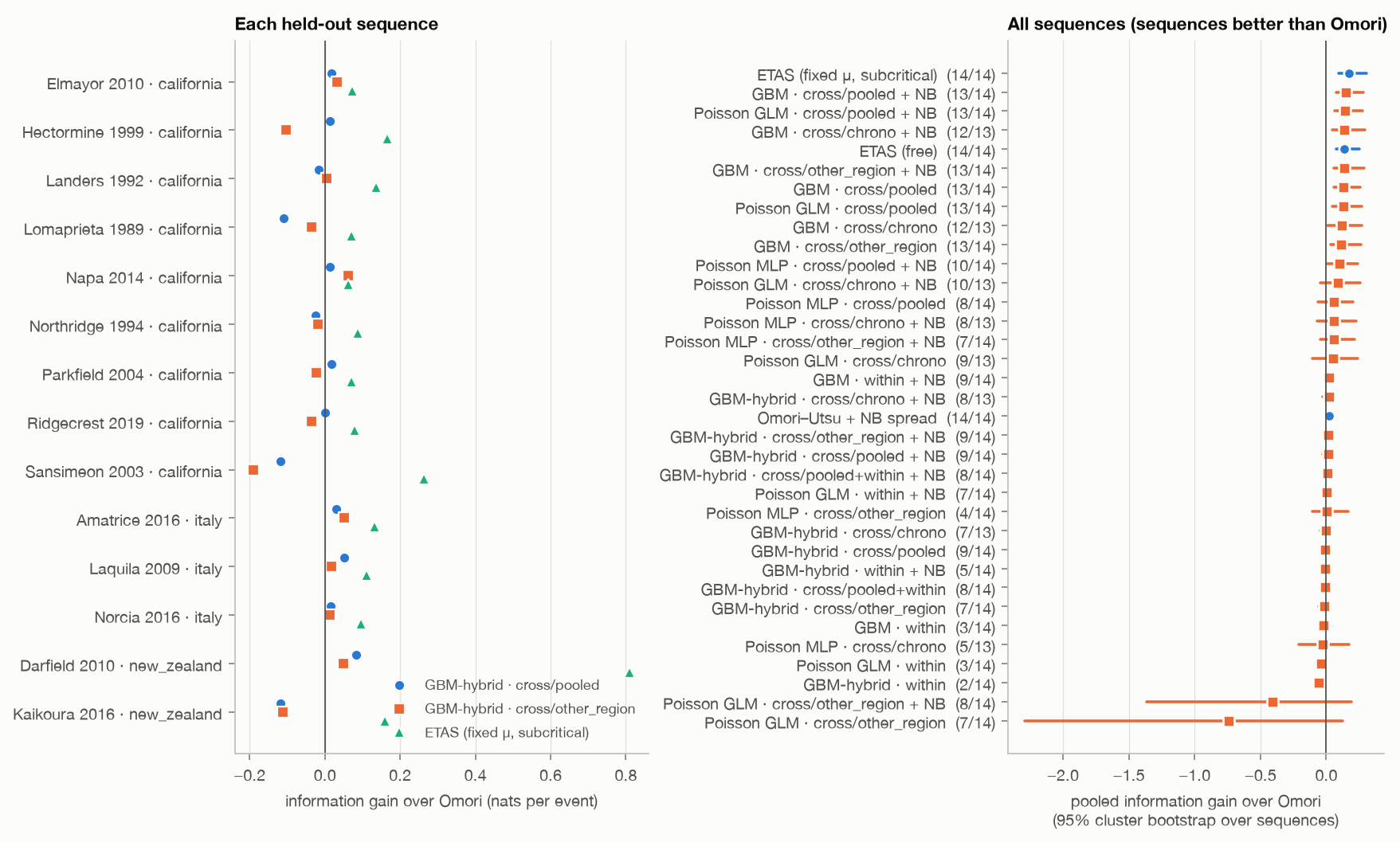
Figure 2. Pooled information gain over Omori–Utsu for every model; 95 % intervals resample whole sequences.
Each sequence was forecast by learned models trained on the others (§4.2), and every model was scored on identical windows. Table 2 gives the per-sequence information gain over Omori–Utsu; intervals below resample whole sequences.
ETAS is the strongest model. It gains +0.171 nats per event ([+0.096, +0.307]) and is above Omori on 14 of 14 sequences. Giving Omori a negative-binomial spread fitted to its own closed forecasts gains only +0.019 ([+0.012, +0.030]), so ETAS's margin is not a dispersion artefact: measured against that recalibrated Omori it is still +0.152 ([+0.080, +0.277]).
Learning across sequences helps; learning within one does not. Gradient boosting and a Poisson GLM trained on the other sequences gain +0.130 ([+0.055, +0.256]) and +0.129 ([+0.048, +0.270]), each above Omori on 13 of 14 sequences, and keep their gain against recalibrated Omori when given the same spread (GBM +0.128, [+0.059, +0.256]). The Poisson MLP is positive but uncertain (+0.059, [−0.061, +0.201]). The same booster trained only on earlier windows of the target sequence loses to Omori (−0.056, [−0.078, −0.030], above it on 2 of 14 sequences), and stays below recalibrated Omori on 0 of 14 when given the spread.
Anchoring to Omori removes the gain. The hybrid booster, which learns a multiplicative correction to the Omori forecast, is indistinguishable from Omori whatever it is trained on: −0.007 ([−0.043, +0.024]) pooled. §7.4 shows why: the learned advantage lives exactly where the Omori fit it is anchored to is broken.
| Sequence | ETAS | Omori + NB | GBM-hybrid (within) | GBM (cross) | GLM (cross) | MLP (cross) | GBM-hybrid (cross) |
|---|---|---|---|---|---|---|---|
| Landers 1992 | +0.135 | +0.016 | −0.019 | +0.083 | +0.080 | +0.094 | −0.016 |
| Hector Mine 1999 | +0.165 | +0.020 | +0.018 | +0.079 | +0.103 | −0.008 | +0.013 |
| Ridgecrest 2019 | +0.078 | +0.009 | −0.092 | +0.070 | +0.044 | +0.034 | +0.000 |
| Northridge 1994 | +0.088 | +0.007 | −0.087 | −0.047 | −0.248 | −0.608 | −0.025 |
| El Mayor–Cucapah 2010 | +0.073 | +0.011 | +0.019 | +0.073 | +0.078 | +0.025 | +0.018 |
| Loma Prieta 1989 | +0.070 | +0.017 | −0.001 | +0.052 | +0.057 | +0.034 | −0.110 |
| San Simeon 2003 | +0.263 | +0.004 | −0.035 | +0.252 | +0.260 | +0.248 | −0.118 |
| South Napa 2014 | +0.061 | +0.034 | −0.035 | +0.092 | +0.134 | −0.069 | +0.012 |
| Parkfield 2004 | +0.071 | +0.009 | −0.009 | +0.002 | +0.040 | −0.155 | +0.018 |
| L’Aquila 2009 | +0.111 | +0.021 | −0.091 | +0.072 | +0.084 | +0.064 | +0.051 |
| Amatrice 2016 | +0.133 | +0.012 | −0.083 | +0.068 | +0.091 | −0.132 | +0.030 |
| Norcia 2016 | +0.095 | +0.028 | −0.086 | +0.063 | +0.056 | +0.055 | +0.016 |
| Darfield 2010 | +0.810 | +0.070 | −0.114 | +0.777 | +0.788 | +0.771 | +0.084 |
| Kaikōura 2016 | +0.160 | +0.007 | −0.068 | +0.021 | +0.040 | −0.114 | −0.119 |
| pooled | +0.171 | +0.019 | −0.056 | +0.130 | +0.129 | +0.059 | −0.007 |
| above Omori | 14 / 14 | 14 / 14 | 2 / 14 | 13 / 14 | 13 / 14 | 8 / 14 | 9 / 14 |
Table 2. Information gain over Omori–Utsu (nats per event) for each held-out sequence; the pooled row weights sequences by their events, and the last row counts sequences above Omori.
7.4 When learning helps
Splitting the pooled score by forecast origin (Table 3, Figure 3) locates every learned gain.
The first three days. Here the Omori fit finished on a search bound in 15 of 42 windows: the catalog is still recovering from short-term incompleteness, the observed rate looks flat, and the sequence cannot identify its own decay parameters. Models that borrow from other sequences gain most: gradient boosting +0.243 ([+0.117, +0.483]), the GLM +0.238, the MLP +0.175. ETAS gains a similar amount (+0.287, [+0.153, +0.533]) by a different route — a structural model that separates the mainshock's direct aftershocks from secondary triggering.
After the first week the gain is gone. At 5–14 days, boosting alone is no longer distinguishable from Omori (+0.019, [−0.021, +0.071]) and Omori with an honest spread matches it (+0.038). From 90 to 240 days boosting is worse than Omori (−0.074, [−0.170, −0.023]), while recalibrated Omori stays ahead (+0.065).
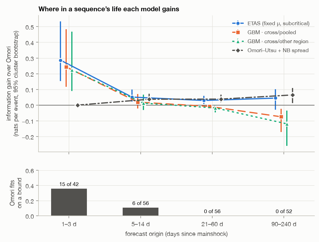
Figure 3. Information gain by forecast origin (top) and the share of Omori fits on a search bound (bottom).
The pattern is the study's central result: machine learning improves aftershock-rate forecasts where — and apparently because — the statistical law cannot yet be fitted to the sequence at hand, and not otherwise.
| Model | 1–3 d | 5–14 d | 21–60 d | 90–240 d |
|---|---|---|---|---|
| ETAS | +0.287 [+0.153, +0.533] | +0.051 [+0.022, +0.099] | +0.030 [+0.007, +0.059] | +0.045 [−0.028, +0.102] |
| Omori + NB | +0.000 [+0.000, +0.000] | +0.038 [+0.017, +0.072] | +0.038 [+0.017, +0.067] | +0.065 [+0.013, +0.110] |
| GBM-hybrid (within) | — | −0.063 [−0.092, −0.031] | −0.033 [−0.064, −0.005] | −0.100 [−0.293, −0.002] |
| GBM (cross, pooled) | +0.243 [+0.117, +0.483] | +0.019 [−0.021, +0.071] | −0.008 [−0.026, +0.004] | −0.074 [−0.170, −0.023] |
| GLM (cross, pooled) | +0.238 [+0.099, +0.480] | +0.016 [−0.024, +0.073] | −0.003 [−0.018, +0.010] | −0.009 [−0.043, +0.015] |
| MLP (cross, pooled) | +0.175 [+0.014, +0.427] | −0.066 [−0.187, +0.034] | −0.069 [−0.153, −0.010] | −0.072 [−0.174, +0.001] |
| GBM-hybrid (cross, pooled) | −0.013 [−0.087, +0.046] | +0.003 [−0.011, +0.015] | −0.006 [−0.024, +0.008] | +0.003 [−0.033, +0.038] |
| Omori fit on a bound | 15 of 42 | 6 of 56 | 0 of 56 | 0 of 52 |
Table 3. Pooled information gain over Omori–Utsu by forecast origin, with 95 % intervals resampling whole sequences, and the share of Omori fits that finished on a search bound.
7.5 Across regions
The strongest test of generalisation trains only on other regions. Early in a sequence it costs little: boosting trained outside the target's region gains +0.224 ([+0.090, +0.469]) in the first three days, against +0.243 for pooled training. Over whole sequences, the event-weighted gain for Californian targets falls from +0.080 to +0.060 and for Italian targets from +0.067 to +0.054. Late in a sequence out-of-region training fails clearly: −0.119 ([−0.259, −0.035]) at 90–240 days.
Two cautions bound this. Region and catalog are confounded — each region's sequences come from a different agency, network and magnitude practice — so "transfers across regions" also means "transfers across catalogs", and the two cannot be separated here. And New Zealand contributes only 2 sequences, where every model's gain over Omori is large (ETAS +0.645) because Omori itself fits those sequences poorly; the regional means for New Zealand should not be read as a property of the region.
7.6 Space
Scored by mean log density at the epicentres that followed, against an adaptive kernel density estimate of past epicentres, the cell-level boosted model gains +0.045 ([−0.019, +0.106]) and is ahead on 6 of 14 sequences — not a reliable improvement. A fixed-bandwidth kernel is worse than the adaptive one (−0.101), and the ETAS-style kernel, a sum of isotropic point sources weighted by expected offspring, is far worse (−0.768, [−0.906, −0.612], behind on every sequence). The density maps show why: a M7 rupture is tens of kilometres of fault, and a point source at the epicentre spreads its offspring into an isotropic blob, while past epicentres already trace the fault.
7.8 Answers to the five questions
- Does spatiotemporal ML improve aftershock-rate prediction? Yes when trained across sequences, and only in the first days of a sequence; it does not beat a dispersion-honest Omori law after about a week, and learning within a single sequence never helps.
- Does it improve spatial density estimation? Not reliably: the boosted model's gain over an adaptive kernel estimate has an interval that includes zero.
- How does it compare with classical models? ETAS is the best single forecaster over the whole window; the best learned model matches ETAS only early, where both exploit what a lone Omori fit cannot.
- How stable are the results across sequences? ETAS is ahead of Omori on every sequence; cross-sequence boosting on 13 of 14; within-sequence learning on 2 of 14. The ordering survives the robustness sweep (§7.7).
- Does generalisation fail across tectonic regimes? Early in a sequence, no — models trained only on other regions keep most of their gain. Late in a sequence, yes. Region and catalog are confounded throughout.
7.7 Robustness
Each of 52 sweep runs changed one design choice (Table 4); 51 completed. The failure is informative: without the truncation rule the Amatrice window runs on through the Norcia sequence, and the ETAS likelihood exceeds the memory cap — the rule is what keeps overlapping sequences apart.
Across the completed runs, ETAS scores above Omori in 42 of 51 (median +0.009) and Omori with the NB spread in 43 of 51 (median +0.019). The within-sequence GBM-hybrid is above Omori in only 14 of 51 (median −0.023). The ordering — dispersion-honest classical models at or above Omori, within-sequence learning at or below it — survives changes to the completeness cutoff, the window start, the zone radius and rule, the window length and the foreshock history. Kaikōura is the exception in the other direction: ETAS falls below Omori under 4 of 4 zone definitions, including a zone twice the Gardner–Knopoff radius.
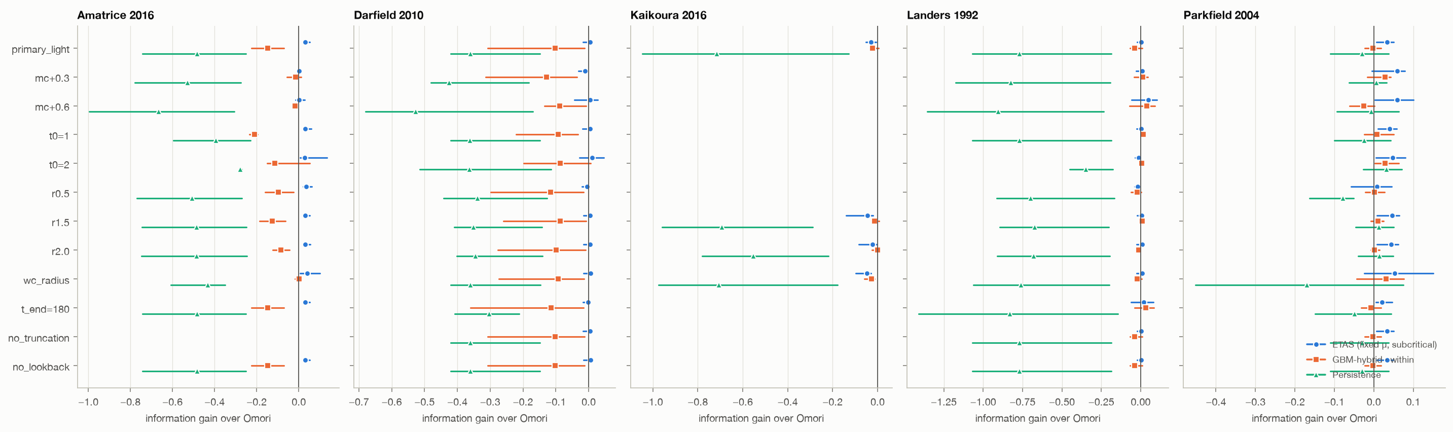
Figure 4. Robustness sweep: information gain over Omori–Utsu under each single-choice variant.
| Sequence | Variant | Mc | Events | ETAS | Omori + NB | GBM-hybrid (within) |
|---|---|---|---|---|---|---|
| Amatrice 2016 | primary_light | 1.8 | 3,912 | +0.030 | +0.032 | −0.149 |
| Amatrice 2016 | mc+0.3 | 2.1 | 1,652 | +0.001 | +0.003 | −0.015 |
| Amatrice 2016 | mc+0.6 | 2.4 | 730 | +0.003 | +0.015 | −0.018 |
| Amatrice 2016 | t0=1 | 1.6 | 5,883 | +0.031 | +0.035 | −0.212 |
| Amatrice 2016 | t0=2 | 1.8 | 3,065 | +0.029 | +0.043 | −0.113 |
| Amatrice 2016 | r0.5 | 1.8 | 3,845 | +0.035 | +0.037 | −0.098 |
| Amatrice 2016 | r1.5 | 1.8 | 3,922 | +0.030 | +0.033 | −0.127 |
| Amatrice 2016 | r2.0 | 1.8 | 3,936 | +0.030 | +0.033 | −0.085 |
| Amatrice 2016 | wc_radius | 1.8 | 2,616 | +0.040 | +0.042 | +0.001 |
| Amatrice 2016 | t_end=180 | 1.8 | 3,912 | +0.030 | +0.032 | −0.149 |
| Amatrice 2016 | no_truncation | failed: MemoryError | ||||
| Amatrice 2016 | no_lookback | 1.8 | 3,912 | +0.030 | +0.032 | −0.149 |
| Darfield 2010 | primary_light | 2.8 | 4,641 | +0.005 | +0.007 | −0.102 |
| Darfield 2010 | mc+0.3 | 3.1 | 2,441 | −0.011 | −0.007 | −0.128 |
| Darfield 2010 | mc+0.6 | 3.4 | 1,242 | +0.005 | +0.016 | −0.088 |
| Darfield 2010 | t0=1 | 2.8 | 4,507 | +0.004 | +0.006 | −0.093 |
| Darfield 2010 | t0=2 | 2.8 | 4,295 | +0.011 | +0.019 | −0.087 |
| Darfield 2010 | r0.5 | 2.8 | 2,945 | −0.005 | −0.004 | −0.116 |
| Darfield 2010 | r1.5 | 2.8 | 4,712 | +0.004 | +0.005 | −0.087 |
| Darfield 2010 | r2.0 | 2.8 | 4,769 | +0.004 | +0.005 | −0.100 |
| Darfield 2010 | wc_radius | 2.8 | 4,645 | +0.006 | +0.007 | −0.093 |
| Darfield 2010 | t_end=180 | 2.8 | 3,217 | −0.002 | −0.001 | −0.114 |
| Darfield 2010 | no_truncation | 2.8 | 4,641 | +0.005 | +0.007 | −0.102 |
| Darfield 2010 | no_lookback | 2.8 | 4,641 | +0.006 | +0.007 | −0.102 |
| Kaikōura 2016 | primary_light | 3.2 | 941 | −0.029 | −0.017 | −0.023 |
| Kaikōura 2016 | r1.5 | 3.3 | 1,021 | −0.046 | −0.005 | −0.014 |
| Kaikōura 2016 | r2.0 | 3.3 | 1,544 | −0.023 | +0.005 | −0.001 |
| Kaikōura 2016 | wc_radius | 3.4 | 802 | −0.048 | −0.032 | −0.027 |
| Landers 1992 | primary_light | 2.5 | 3,679 | +0.002 | +0.012 | −0.039 |
| Landers 1992 | mc+0.3 | 2.8 | 1,644 | +0.011 | +0.026 | +0.013 |
| Landers 1992 | mc+0.6 | 3.1 | 680 | +0.047 | +0.068 | +0.038 |
| Landers 1992 | t0=1 | 2.5 | 3,465 | +0.002 | +0.013 | +0.017 |
| Landers 1992 | t0=2 | 2.5 | 3,153 | −0.012 | −0.000 | +0.006 |
| Landers 1992 | r0.5 | 2.5 | 2,353 | −0.019 | −0.006 | −0.023 |
| Landers 1992 | r1.5 | 2.5 | 4,403 | +0.005 | +0.013 | +0.010 |
| Landers 1992 | r2.0 | 2.5 | 4,487 | +0.011 | +0.019 | −0.011 |
| Landers 1992 | wc_radius | 2.5 | 3,795 | +0.009 | +0.018 | −0.023 |
| Landers 1992 | t_end=180 | 3.0 | 844 | +0.021 | +0.054 | +0.031 |
| Landers 1992 | no_truncation | 2.5 | 3,679 | +0.002 | +0.012 | −0.039 |
| Landers 1992 | no_lookback | 2.5 | 3,679 | +0.003 | +0.012 | −0.039 |
| Parkfield 2004 | primary_light | 1.2 | 2,666 | +0.034 | +0.031 | −0.002 |
| Parkfield 2004 | mc+0.3 | 1.5 | 1,408 | +0.059 | +0.052 | +0.029 |
| Parkfield 2004 | mc+0.6 | 1.8 | 760 | +0.060 | +0.047 | −0.026 |
| Parkfield 2004 | t0=1 | 1.2 | 2,566 | +0.041 | +0.036 | +0.009 |
| Parkfield 2004 | t0=2 | 1.2 | 2,483 | +0.048 | +0.045 | +0.028 |
| Parkfield 2004 | r0.5 | 1.5 | 573 | +0.009 | +0.028 | +0.002 |
| Parkfield 2004 | r1.5 | 1.2 | 4,485 | +0.046 | +0.042 | +0.011 |
| Parkfield 2004 | r2.0 | 1.2 | 4,805 | +0.044 | +0.040 | +0.001 |
| Parkfield 2004 | wc_radius | 1.2 | 590 | +0.053 | +0.060 | +0.031 |
| Parkfield 2004 | t_end=180 | 1.2 | 1,885 | +0.021 | +0.021 | −0.007 |
| Parkfield 2004 | no_truncation | 1.2 | 2,666 | +0.034 | +0.031 | −0.002 |
| Parkfield 2004 | no_lookback | 1.2 | 2,666 | +0.034 | +0.031 | −0.002 |
Table 4. Robustness sweep: information gain over Omori (nats per event) on windows where every model forecast, at light settings (eight origins).
8. Reviewer 2
"The early gain is a catalog artefact." It may be, in part. The learned models win exactly where the catalog is least complete, so what transfers across sequences could be how catalogs recover from short-term incompleteness rather than how aftershock sequences behave. The completeness protocol takes the worst time bin and the window starts at half a day, and raising Mc by 0.3 or 0.6 or delaying the start to one or two days leaves the classical ordering intact (§7.7) — but the design cannot separate learned physics from learned catalog behaviour, and the claim here is only that the learned models forecast the recorded catalog better early on.
"There is leakage." Every forecast uses events up to its origin only; every training window closes before the origin (enforced in code and tested); the target sequence never enters its own cross-sequence pool. Pooled training does include sequences later in calendar time, so a chronological pool (earlier sequences only) was run as a control: early in a sequence it gains +0.231 against +0.243 pooled. The completeness magnitude is set once per sequence from the whole window; it is identical for every model and so cannot favour one.
"The ETAS baseline is weak." It is temporal-only, uses point sources, and is fitted by maximum likelihood rather than with generic prior parameters, as operational systems commonly are. But it is not a strawman: the estimator recovers known parameters, the simulation forecaster is calibrated when given the true parameters, the background rate comes from the pre-mainshock catalog, and it is the best model in this study. Its failures — unidentified early fits and runaway long-horizon cascades — are reported, not tuned away.
"The sequence definition decides the answer." The Gardner–Knopoff circle is a crude zone for multi-fault ruptures; Kaikōura is the clearest case, where ETAS stays below Omori under every zone tried, including twice the radius. Radius, rule and truncation were varied (§7.7) without reversing the main ordering; the one failure (Amatrice without truncation) is reported.
"Fourteen sequences are few, and the regions are unbalanced." Yes. Nine are Californian; New Zealand has two. Intervals resample whole sequences, which is honest about that and makes them wide. Regional statements are made only where the data carry them.
"You tried many models and report the best." Every model variant is reported, including those that lose; hyperparameters were fixed before the cross-sequence run; the pre-registration changes that were made are listed in §6a.
"None of this is operational." Correct. The target is the count of events above a completeness magnitude inside a zone — not the probability of a damaging aftershock — and the gains, while real, are small in absolute terms outside the first days. QuakeCast characterises sequences; it forecasts nothing a warning could be based on. ETAS baseline quality, sequence definition, tectonic heterogeneity, overfitting, operational relevance.
9. Limitations
- Fourteen sequences, three regions, three catalogs. Region and catalog are confounded, and regional results for Italy and New Zealand rest on three and two sequences.
- Counts, not hazard. Every target is a count above Mc in a circular zone; magnitudes of future events, ground motion and damage are out of scope.
- Temporal ETAS only. Rate forecasts use a temporal ETAS; spatial ETAS enters only as a density kernel, with point sources and no rupture geometry.
- Early incompleteness. The first half-day is excluded and early windows remain incomplete at low magnitudes; the learned early gain may partly reflect catalog behaviour (§8).
- Maximum-likelihood fits. No Bayesian or generic-parameter ETAS, which would likely help the early, unidentified fits most.
- Numerical note. Six divide-by-zero warnings appeared in the ETAS gradient during the first wave of robustness runs and could not be reproduced; such points are now rejected by a counted guard, and the affected runs were not repeated.
References
Reference details (volume and pages) are to be checked against the publisher records before any submission.
- Aki, K. (1965). Maximum likelihood estimate of b in the formula log N = a − bM and its confidence limits. Bulletin of the Earthquake Research Institute, University of Tokyo.
- Cao, A., & Gao, S. S. (2002). Temporal variation of seismic b-values beneath northeastern Japan island arc. Geophysical Research Letters.
- Czado, C., Gneiting, T., & Held, L. (2009). Predictive model assessment for count data. Biometrics.
- Gardner, J. K., & Knopoff, L. (1974). Is the sequence of earthquakes in Southern California, with aftershocks removed, Poissonian? Bulletin of the Seismological Society of America.
- Gneiting, T., & Raftery, A. E. (2007). Strictly proper scoring rules, prediction, and estimation. Journal of the American Statistical Association.
- Gutenberg, B., & Richter, C. F. (1944). Frequency of earthquakes in California. Bulletin of the Seismological Society of America.
- Helmstetter, A., Kagan, Y. Y., & Jackson, D. D. (2006). Comparison of short-term and time-independent earthquake forecast models for southern California. Bulletin of the Seismological Society of America.
- Kagan, Y. Y. (2004). Short-term properties of earthquake catalogs and models of earthquake source. Bulletin of the Seismological Society of America.
- Ogata, Y. (1988). Statistical models for earthquake occurrences and residual analysis for point processes. Journal of the American Statistical Association.
- Omori, F. (1894). On the after-shocks of earthquakes. Journal of the College of Science, Imperial University of Tokyo.
- Page, M. T., van der Elst, N., Hardebeck, J., Felzer, K., & Michael, A. J. (2016). Three ingredients for improved global aftershock forecasts: Tectonic region, time-dependent catalog incompleteness, and intersequence variability. Bulletin of the Seismological Society of America.
- Reasenberg, P. A., & Jones, L. M. (1989). Earthquake hazard after a mainshock in California. Science.
- Schorlemmer, D., Gerstenberger, M. C., Wiemer, S., Jackson, D. D., & Rhoades, D. A. (2007). Earthquake likelihood model testing. Seismological Research Letters.
- Shi, Y., & Bolt, B. A. (1982). The standard error of the magnitude-frequency b value. Bulletin of the Seismological Society of America.
- Utsu, T. (1961). A statistical study on the occurrence of aftershocks. Geophysical Magazine.
- Wells, D. L., & Coppersmith, K. J. (1994). New empirical relationships among magnitude, rupture length, rupture width, rupture area, and surface displacement. Bulletin of the Seismological Society of America.
- Wiemer, S., & Wyss, M. (2000). Minimum magnitude of completeness in earthquake catalogs: Examples from Alaska, the western United States, and Japan. Bulletin of the Seismological Society of America.
- Woessner, J., & Wiemer, S. (2005). Assessing the quality of earthquake catalogues: Estimating the magnitude of completeness and its uncertainty. Bulletin of the Seismological Society of America.
- Zechar, J. D., Gerstenberger, M. C., & Rhoades, D. A. (2010). Likelihood-based tests for evaluating space–rate–magnitude earthquake forecasts. Bulletin of the Seismological Society of America.